Finite Differences#

강좌: 기초 전산유체역학

Taylor Expansion#

Taylor series를 이용하면 함수를 쉽게 근사화 할 수 있다.

\[ f(x_j+\Delta x) = f(x_j) + \Delta x f'(x_j) + \frac{(\Delta x)^2}{2} f''(x_j) + \frac{(\Delta x)^3}{3!} f'''(x_j) + T.E. \]

여기서 \(T.E\) 는 Truncation error 이다. 만약 1차 미분까지만으로 근사화 한 경우 이 오차는 \((\Delta x)^2, (\Delta x)^3, ...\) 과 같이 간격 \(\Delta x\) 의 고차 항으로 구성되어 있다.

\[ T.E. = Error((\Delta x)^2, (\Delta x)^3, ...) = O((\Delta x)^2) \]

\(\Delta x\) 가 작은 경우 오차는 Leading error 항과 그보다 매우 작은 항의 합이다.

수치 미분#

Forward, Backward, Central differences#

fd-fig — Fig. 7 Finite Difference (from Wikipedia)#

Forward Difference

\[ f'(x_j) = \frac{f(x_{j+1}) - f(x_j)}{\Delta x} + O(\Delta x) \]
Backward Differnce

\[ f'(x_j) = \frac{f(x_{j}) - f(x_{j-1})}{\Delta x} + O(\Delta x) \]
Central Difference
- 다음 두 식을 빼보자.
  
  \[ f(x_{j+1}) = f(x_j) + \Delta x f'(x_j) + \frac{(\Delta x)^2}{2} f''(x_j) + \frac{(\Delta x)^3}{3!} f'''(x_j) + O((\Delta x)^4) \]
  
  \[ f(x_{j-1}) = f(x_j) - \Delta x f'(x_j) + \frac{(\Delta x)^2}{2} f''(x_j) - \frac{(\Delta x)^3}{3!} f'''(x_j) + O((\Delta x)^4) \]
- 그 결과는 다음과 같다.
\[ f'(x_j) = \frac{f(x_{j+1}) - f(x_{j-1})}{ 2\Delta x} + O((\Delta x)^2) \]
- 위의 두 식을 더한 후 \(2 f(x_j)\) 를 빼보자.
\[ f''(x_j) = \frac{f(x_{j+1}) - 2 f(x_j) + f(x_{j-1})}{ (\Delta x)^2} + O((\Delta x)^2) \]

One-sided difference#

\(j, j-1 j-2\) 점을 기준할 때 차분식이 다음과 같다고 생각하자.

\[ f'(x_j) = \frac{a f(x_j) + b f (x_{j-1}) + c f(x_{j-2})}{\Delta x} + TE \]
- 다음 수식을 대입하면
\[ f(x_{j-1}) = f(x_j) - \Delta x f'(x_j) + \frac{(\Delta x)^2}{2} f''(x_j) - \frac{(\Delta x)^3}{3!} f'''(x_j) + O((\Delta x)^4) \]

\[ f(x_{j-2}) = f(x_j) - 2 \Delta x f'(x_j) + \frac{(2 \Delta x)^2}{2} f''(x_j) - \frac{(2 \Delta x)^3}{3!} f'''(x_j) + O((\Delta x)^4) \]
- 분자는 다음과 같다.
\[ (a + b + c) f(x_j) - \Delta x (b + 2c) f''(x_j) + \frac{(\Delta x)^2}{2} (b + 4c) f''(x_j) + O(\Delta x^3) \]
- 즉 다음을 만족해야 한다.
\[\begin{split} \begin{align} a + b + c &= 0 \\ b + 2c &= -1 \\ b + 4c &= 0 \end{align} \end{split}\]
- \(a=3/2, b=-2, c=1/2\).
\[ f'(x_j) = \frac{3 f(x_j) -4 f (x_{j-1}) + f(x_{j-2})}{2 \Delta x} + O(\Delta x^2) \]
(DIY) 같은 Stencil (계산점)에서 \(f''(x_j)\) 차분식을 구하고 그 정확도를 비교하시오.

일반적인 방법#

여러 Taylor expansion의 합차를 이용해서 원하는 미분항의 근사식을 구한다.

예제#

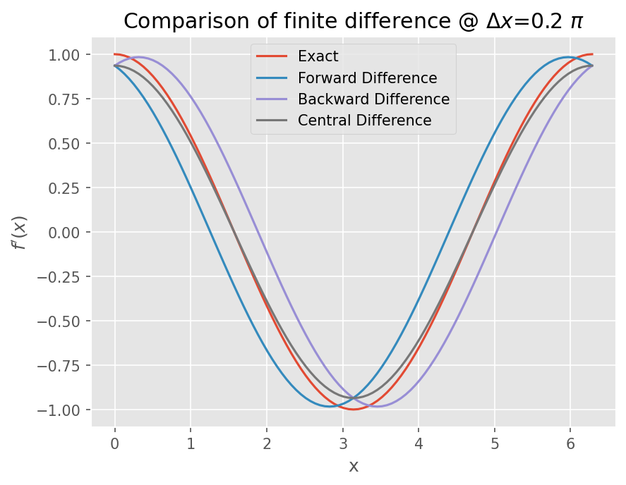
\(f(x)=\sin(x)\) 에 대해서 수치 미분 결과를 비교하자.

%matplotlib inline
from matplotlib import pyplot as plt

import numpy as np

plt.style.use('ggplot')
plt.rcParams['figure.dpi'] = 150

def forward_diff(f, x, dx):
    """
    Forward Difference
    ------------------
    
    Parameters
    ----------
    f : function
        Function being differentiated
    x : float
        Point where derivative is approximated
    dx : float
        Step size
        
    Return
    ------
    df : float
        Value by forward difference
    """
    return (f(x+dx) - f(x)) / dx

def backward_diff(f, x, dx):
    """
    Backward Difference
    ------------------
    
    Parameters
    ----------
    f : function
        Function being differentiated
    x : float
        Point where derivative is approximated
    dx : float
        Step size
        
    Return
    ------
    df : float
        Value by backward difference
    """
    return (f(x) - f(x-dx)) / dx

def central_diff(f, x, dx):
    """
    Central Difference
    ------------------
    
    Parameters
    ----------
    f : function
        Function being differentiated
    x : float
        Point where derivative is approximated
    dx : float
        Step size
        
    Return
    ------
    df : float
        Value by central difference
    """
    return (f(x+dx) - f(x-dx)) / (2*dx)

def compute(dx):
    # Sine function at [0, 2 \pi]
    x = np.linspace(0, 2*np.pi, 101)
    f = np.sin

    # Compute first derivatives
    exact = np.cos(x)
    fd = np.array([forward_diff(f, xi, dx) for xi in x])
    bd = np.array([backward_diff(f, xi, dx) for xi in x])
    cd = np.array([central_diff(f, xi, dx) for xi in x])
    
    # points, exact value, forward / backward / central dfference
    return x, exact, fd, bd, cd

def plot(dx):
    # Results of foward, backward, central differences 
    x, exact, fd, bd, cd = compute(dx)

    # Plot exact, forward, backward, central difference
    plt.plot(x , exact)
    plt.plot(x, fd)
    plt.plot(x, bd)
    plt.plot(x, cd)
    
    # Legend, labels, title
    plt.legend(['Exact', 'Forward Difference', 'Backward Difference', 'Central Difference'])
    plt.xlabel(r'x')
    plt.ylabel(r"$f'(x)$")
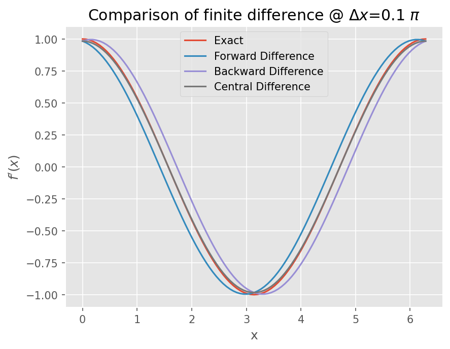
    plt.title("Comparison of finite difference @ $\Delta x$={} $\pi$".format(dx/np.pi))

plot(0.2*np.pi)

../_images/aef1b7ca18770b90b785476fdcffac059b194b3cffb22ccdbba0bfd272b426af.png

plot(0.1*np.pi)

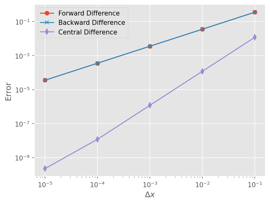
../_images/7a5d2fee797d45872c1d23402fe94eb001ee3ea6391e385b6418ea95325c9074.png

정확도 비교#

Forward / Backward difference 는 1차 정확도 (\(O(\Delta x)\))
Central difference 는 2차 정확도(\(O((\Delta x)^2)\))

def error(dx):
    # Results of foward, backward, central differences 
    _, exact, fd, bd, cd = compute(dx)
    
    # Compute error norm
    err_fd = np.linalg.norm(fd - exact) 
    err_bd = np.linalg.norm(bd - exact) 
    err_cd = np.linalg.norm(cd - exact) 
    
    return err_fd, err_bd, err_cd

# Change delta x
dxs = [10**(-n) for n in range(1, 6)]

err_fd, err_bd, err_cd = [], [], []

for dx in dxs:
    fd, bd, cd = error(dx)
    
    err_fd.append(fd)
    err_bd.append(bd)
    err_cd.append(cd)    
    
# Plot error (log-log scale)
plt.loglog(dxs, err_fd, marker='o')
plt.loglog(dxs, err_bd, marker='x')
plt.loglog(dxs, err_cd, marker='d')

plt.legend(['Forward Difference', 'Backward Difference', 'Central Difference'])
plt.xlabel(r'$\Delta x$')
plt.ylabel('Error')

Text(0, 0.5, 'Error')

../_images/1b2428d7df0449dda81bdc164a7127adcc4c2bf160b0ba732db13a7de06b923d.png

과제#

다음 1차 미분 근사식에 대해 오차의 정확도를 분석하고, 수치적으로 검증하시오.

\[ f'(x) = \frac{3 f_i - 4 f_{i-1} + f_{i-2}}{2 \Delta x} \]

다음 2차 미분 근사식에 대해 오차의 정확도를 분석하고, 수치적으로 검증하시오.

\[ f''(x) = \frac{- f_{i+3} + 4 f_{i+2} - 5 f_{i+1} + 2 f_{i}}{\Delta x^2} \]

Finite Differences

Contents